A new method for determining the shape of the sclera
Purpose: The aim of the present theoretical modelling study is to improve the fitting of scleral lenses by means of a novel determination of the scleral shape of the eye.
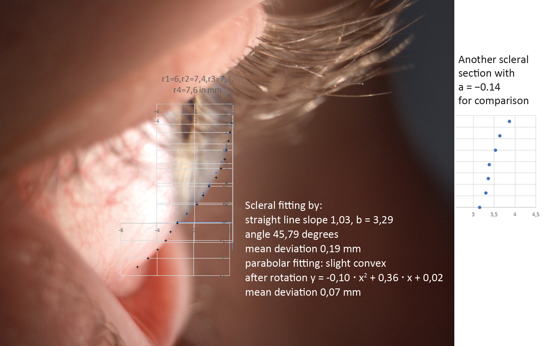
Material and Methods: The movement of scleral lenses and soft lenses is affected by scleral shape around the limbus. Based on this, it is important to take a closer look at the edge of the sclera. An area of 4 mm in diameter around the limbus is considered as a suitable area for shape fitting, which is shown by 44 profile photographs. As a first step, a straight line (y = m • x + b) was fitted on scleral data of 44 perpendicular cuts. Then, these measuring points were rotated around the first “scleral measuring point after the limbus” (angle of rotation = − arctan (m)) so that all measuring points were horizontal. A parabola was then fitted as best as possible (y = a • x2 + b • x + c) to the rotated measuring points. The parabola coefficient a or “pca value” plays a central role as a shape criterion of the corneo-scleral profile (CSP). A pca value a ≥ 0.1 means the CSP is a concave parabola, while a ≤ −0.1 implies that the CSP is a convex one. If the pca value is between −0.1 < a < 0.1, the CSP is a straight line.
Results: Based on the 44 profile section photos, 85.8 % of the CSPs were straight, 11.1 % were convex and 3.1 % were concave parabolic shapes. The probability of determining a parabolic CSP section is about 18.5 % (normal distribution, the normal distribution test for the calculated pca values shows p < 0.01).
Conclusion: A specification of the corneo-scleral-profile (CSP) with the corresponding scleral angle alpha, gives significantly more information about the scleral shape than if only one of the two parameters is specified. Furthermore, this simplifies the determination of the geometry of contact lenses with large diameters, especially scleral lenses.
Introduction
A rigid mini-scleral lens has an overall diameter between 11.5 mm and 15.5 mm.1 Rigid scleral lenses sit on the sclera with the haptic zone of the lens. Soft lenses should extend beyond the limbus and have a standard diameter between 13.0 mm and 14.5 mm, depending on the type: daily, monthly, yearly contact lens, toric or spherical.2
For soft and scleral lens fittings, a scleral shape description is interesting because the shape of the lens is influenced by the scleral fit.3,4,5
The corneal diameter, which is important in this context, is approximately 11.7 mm horizontally and 10.6 mm vertically on average in Europe.6
Gaggioni and Meier first described the corneo-scleral profile of the eye in 1987 in the context of fitting soft contact lenses and differentiated between fluid convex, fluid tangential, fluid concave, marked convex and marked tangential.7 Based on this, optometrists in the German-speaking regions of Europe in particular became involved early on with fitting soft contact lenses based on the determination of the corneo-scleral profile.8,9 The current state of knowledge on the topography of the sclera was discussed by Gier et al. and Bandlitz, among others.10,11
This paper describes a new method to computationally determine the scleral shape of the eye and the angle of inclination.
In order to be able to discuss the profiles in more detail, it is suitable to consider a straight-line fitting for the tangential profiles and a parabolic fitting for the convex and concave profiles on the sclera.
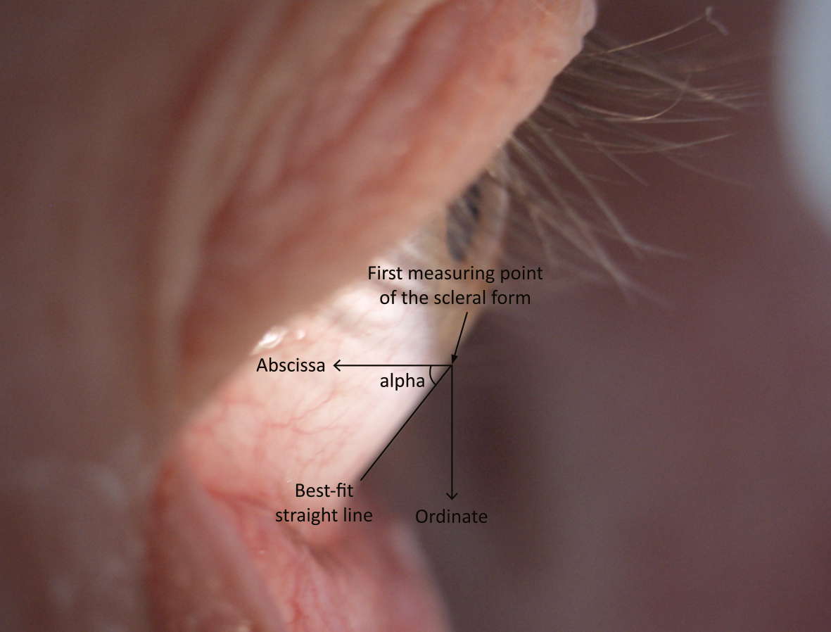
Furthermore, it is useful to describe the slope of the sclera expressed by the scleral angle (here angle alpha). The scleral angle alpha is the one formed between the best-fit straight line of the Corneo-Scleral Profile (CSP) and the x-axis of a coordinate system with the origin of the first measuring point on the sclera after the limbus. The x-axis is also parallel to the optical axis of the eye (Figure 3). First, a side profile image was taken of the upper half and then of the lower half of the eye under observation. The subject was presented with distance optotypes during the exposure to ensure straight-ahead vision.
Material and methods
The linear equation y = m • x + b and the parabolic equation y = a • x2 + b • x + c were each best fitted to the data from the side profile images taken from the eyes of 11 subjects between 22 and 48 years of age; this is a total of 44 independent scleral shape fits (22 eyes with upper and lower side profile images, respectively). Verbal informed consent was obtained from the subjects for the use of their anonymised data. Exclusion criteria were any form of intraocular and/or corneal surgery. A Zeiss SL 120 slit lamp with a 10-fold magnification was used for the images. Starting from the first measurement point on the sclera, a profile length of approximately 4 mm was measured on the sclera and measurement points were obtained at 0.25 mm intervals on the y-axis of the coordinate system described previously (Figure 3). The considered scleral width of 4 mm is based on the following consideration: With a corneal diameter of ~ 12.0 mm and a lens diameter of ~ 16.0 mm and assuming a central fil, the lens edge protrudes 2 mm beyond the cornea. With a safety margin of 2 mm due to lens movement, a scleral width of 4 mm should be reasonable (Figure 1).5,12
First, a mean straight-line fitting was calculated. The programme Excel was used together with mathematics analysis tool Octave (Octave is implemented in C++) and the principle of Gaussian least squares was applied to fit the straight lines. The quality of the straight-line fitting was checked with the average deviation between the measuring points and the calculated points of the fitted straight line.13
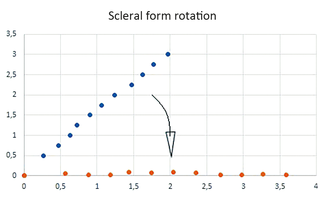
The angle alpha was determined using the slope of the best-fit straight line. The angle alpha is the angle between the x-axis and the best-fit straight line with intersection in the first point of the description of the scleral shape (Figure 3). The angle alpha was calculated with the arctan of the straight-line slope m. To fit the data to a parabola, the scleral measuring points are first rotated around the first measuring point of the scleral form with −alpha with the help of a rotation matrix, whereby the best-fitted straight line of all scleral measuring points is then located horizontally on the x-axis (Figure 2, Figure 3). This has the advantage that the general parabolic equation can be used to fit the rotated scleral measuring points.
Using the rotated measuring points, a parabola was fitted using the Gaussian least squares principle. The coefficients of the parabola equation were determined via the first partial derivative of each parabola coefficient.13 Here, the mean deviation of the calculated parabolic equation from the scleral measuring points was used as a quality control. The differences between the pairs of measured values, e. g. xi;yi and the corresponding function values of the parabola f(xi) = a • xi2 + b • xi + c were formed. yi − f(xi) was then squared and the difference squares were added up.
In order to assess theoretical modelling, two experienced clinicians used the anonymised digital photographs of the corneo-scleral profile (CSP). A comparison of the shape of the CSP was made with external shape descriptions and not with fitted contact lenses. Due to the study design, ethics committee approval was not required.
Mathematical consideration of parabolic fitting 13
According to the principle of Gaussian squares, the difference vi between the y-value of the measuring point and the corresponding y-value of the parabola must result in a minimum:
S(a,b,c) = ∑in vi2 = ∑in (yi − a • xi2 − b • xi − c)2 →Minimum
The 1st order partial derivative of S(a,b,c):
∂S ⁄ ∂a = 2 • ∑i=1n (yi − a • xi2 − b • xi − c)1 • (−xi2) = 0
∂S ⁄ ∂b = 2 • ∑i=1n (yi − a • xi2 − b • xi − c)1 • (−xi) = 0
∂S ⁄ ∂c = 2 • ∑i=1n (yi − a • xi2 − b • xi − c)1 • (−1) = 0
We have here a system of linear equations that can be solved with Cramer‘s rule.
(∑i=1n xi4) • a + (∑i=1n xi3) • b + (∑i=1n xi2) • c = (∑i=1n xi2 • yi)
(∑i=1n xi3) • a + (∑i=1n xi2) • b + (∑i=1n xi) • c = (∑i=1n xi • yi)
(∑i=1n xi2) • a + (∑i=1n xi) • b + n • c = (∑i=1n yi)
The parabola coefficient a represents the quadratic part of the parabola equation. If the coefficient a is close to zero, the quadratic part of the parabolic function is negligible, and the shape formed by the scleral measuring points is fairly well described by a straight line. Conversely, if the coefficient is significantly different from zero, the shape formed by the scleral measuring points can be described with a parabola.
The conjunctiva has at least two layers of non-keratinised epithelial cells in the area under consideration; the thickness is therefore likely to be more than 20 μm. Since the conjunctiva is variable in thickness and soft, a higher accuracy of more than 0.02 mm is therefore unlikely to be useful.14,15,16
Results
Coefficient Tolerances
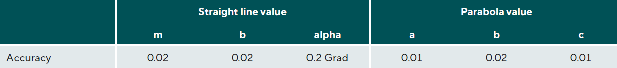
To check how accurately the straight-line fitting or parabolic fitting could be carried out, five CS profiles were each recorded four times, and a scleral fitting was carried out in each case. Once the pca values and angles were obtained, the respective deviations were determined according to a Bland-Altman plot and these are shown as tolerances in Table 1.17
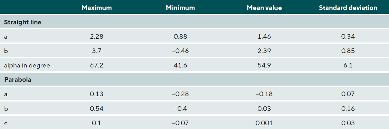
The tolerances described above were then used as the basis for rounding the digits of the data presented in Table 2. The following features emerged:
- The slope coefficient m and the corresponding scleral angle alpha vary greatly. This means that the scleral angle alpha or the slope m should be an integral metric of the CSP shape description.
- The low values of the parabola coefficient c are due to the following: The measuring points are rotated around the first scleral measuring point (zero point of the coordinate system with which the scleral measuring points are described) to the x-axis. The measuring points are then approximately horizontal and thus a low value c is expected.
- pca values that are significantly above +0.1 and below −0.1 describe a marked parabolic shape.10
The pca value of the parabola equation served as a decision criterion as to whether the scleral curvature in the 4 mm zone can be approximately classified as a straight line or a parabola. 44 perpendicular sections were viewed independently by two clinicians and it was noticed that a clearly visible scleral curvature is present from a pca value of a ≥ +0.1; this is then a concave CSP and a ≤ −0.1 corresponds to a convex CSP in this case (Figure 1). For a straight CSP, the coefficient is then between −0.1 < a < 0.1. In practice, the scleral shape is often determined with the slit lamp. With the described pca values, the proportion of straight line fittings is best in line with our practical experience.
If the values a ≥ +0.1 and a ≤ -0.1 are taken as criteria for CSP shape determination, 3.1 % of the 44 profiles are greater than or equal to +0.1 and 11.1 % are less than or equal to −0.1. The probability of measuring a parabolic shape is 18.5 % (pca values are normally distributed, normal distribution test p < 0.01).
Discussion
The basic idea of the method described in this paper is to describe the shape of the sclera according to Gaggioni and Meier in connection with the scleral angle alpha. If the edge of a lens lies on a convex or on a concave sclera, a different fit should be expected. If we further assume, for example, a tangential scleral shape, the scleral angle should also be important for a proper fit. If the range of the angle alpha is small, it is worth considering to only take the scleral shape description according to Gaggioni and Meier into account.7
In this study, the mean angle alpha is 54.9 degrees and the range of the angle alpha is 25.6 degrees for all collected CSP measurement data, both superior and inferior (Table 2). Each CS eye profile, independently of it being superior, inferior, temporal or nasal, is different. For example, Bandlitz described the nasal CSP span as 3.0 degrees (OCT measurements) in a study by Ritzmann et al. and 2.9 degrees (Scheimpflug measurements) in a study by Gier et al.10 The data show that it makes sense to specify the CSP shape together with the corresponding scleral angle, since we then get more information for lens fitting. Other studies give information on the scleral shape; Gaggioni and Meier described a straight-line percentage of 58.8 % (slit lamp measurement) and Rott-Muff et al. a straight-line percentage of 48.8 % (slit lamp measurement) in this context.7,18 The straight-line fraction sometimes depends on the selected CSP width. If the CSP width under consideration is increased, the CSP may well become concave or convex if it was previously straight. A larger CSP width should therefore produce a different result.
Furthermore, the „pca value decision criterion“ of ±0.1 is important in this described method. This criterion was subjectively determined in this study by two experienced contact lens fitters; it was not validated. Such a validation should be carried out in a follow-up study to confirm or slightly adjust this criterion upwards or downwards due to the limited amount of measurement data available here.
With the given criteria, the average slope in this study is 1.46, (Table 2); the best-described shape of the CSP here is a straight line in most cases (85.8% with a CSP width of 4 mm). 11.1 % of the results exhibited a convex parabolic shape, whereas 3.1 % were concave parabolic.
Conclusion
The method described here might seem a bit complicated, but the described calculations of the scleral shape and the corresponding scleral angle can easily be integrated into an analysis programme. This way, it is possible to not only obtain the angle alpha of the CSP shape at different positions, but also the CSP shape itself. If it is a convex shape or a concave shape, we can also get information about the degree of curvature. This is well expressed by the value of the parabola coefficient a („pca value“). This opens up valuable additional information for contact lens fitting. An indication of the CSP shape together with the corresponding scleral angle alpha gives much more information than if only one of the two values is given.
Furthermore, the results of this method can easily be analysed statistically. The conjunctiva is a very soft layer; if the contact lens is placed parallel to it, this can avoid irritation. Thus, the method described helps to determine the best first fitting lens possible, which in turn has a positive influence on the comfort level of lens wear after putting on the lens for the first time. Additional studies would be helpful to test the pca value considerations described here in clinical practice in more detail.
Conflict of interest
The author has no conflict of interest in relation to the methods and devices mentioned in this article.
Figures: Copyright by Manfred Bufler
Article for download
Download here: A new method for determining the shape of the sclera